Minimizers
What is a minimizer?
A minimizer is an optimisation algorithm or heuristic which takes a set of input parameters and a function of the inputs, and aims to find which combination of inputs makes the result of the function the smallest (minimal).
Example: Gradient Descent
To visualise a minimizer, picture a hilly terrain. The minimizer is trying to find the lowest valley in this terrain (the global minimum). For this example, our initial parameters can be pictured as the position of a ball on this terrain. Gradient descent does this by rolling the ball down the steepest path it can find, stopping and reassessing (i.e. without momentum) at regular intervals. (note here, that the valley we start in may not be the deepest valley in the landscape and we may only find the bottom of the valley we started in, the local minimum, initial parameters are key) Other minimizers might be pictured as an (or many) automata moving around trying to find the lowest valley; many minimizers are based on a concept of a ‘walk’.
The gradient descent algorithm proceeds as follows:
Start at some position.
Calculate the gradient, or slope, of the current location.
Take a step (of some fixed size) in the direction where the slope goes downhill the steepest.
Repeat from to step 2 until reaching a equilibrium point (a point where the gradient is zero in all directions).
Through this, the minimizer is guaranteed to end up at the bottom of some valley. However, if it ends up at the bottom of a valley, it has no way of knowing whether it’s the deepest in all the land, and it is stuck down there. More complicated algorithms have ways of dealing with this.
Nonetheless, this is an example of minimization; our inputs are the x and y coordinates of the minimizer’s current position, and the output is their altitude at that location. We call the space of all possible combinations of inputs the “parameter space”, and the output function the “objective function” (objective as in ‘goal’ or ‘target’).
Minimization is a huge field of mathematics, and many more sophisticated algorithms exist. Popular, ubiquitous minimization algorithms include the Levenberg-Marquardt algorithm or the BFGS algorithm.
How does MDMC use minimization?
MDMC’s parameter space for minimization are the parameters governing the interactions between molecules in a given simulation. It aims to minimize the Figure of Merit (FoM) between a simulation using those parameters and experimental data. Through this, it finds the parameters which create a simulation that most closely reproduces the experimental data.
Derivative-free optimisation
Many fast minimization algorithms, such as the ones above, rely on being able to calculate the slope or gradient of the objective function. However, MDMC’s objective function (the figure of merit) is based on the difference between experimental and simulated data. Both experimental data and molecular dynamics simulations are noisy, which makes the figure of merit ‘not smooth enough’ to use many of these algorithms; the idea of a ‘slope’ does not make sense!
We thus turn to ‘derivative-free optimisation’, which is a subfield of optimisation that avoids needing gradient information. Derivative-free optimisation is also known as ‘black-box optimisation’; the objective function is a ‘black-box’, where we do not have some mathematical formula for it.
We will now detail the minimizers available in MDMC.
Covariance Matrix Adaptation Evolution Strategy
The CMA-ES package provides an optimisation algorithm which generates the parameters within a given standard deviation around the initial values, and determines their covariance matrix based on the calculated values at each point. This approach requires a larger number of function evaluations before convergence is reached. At the same time, it can handle noisy data and functions with local minima.
Gaussian Process Regression
The Gaussian Process Regression (GPR) algorithm aims not to minimize, but to ‘map out’ parameter space. It first creates a grid of values in parameter space and calculates the objective function at each of these points. It uses these values to ‘fit’ an approximate topography to the space, and then predicts the values between by interpolation via a defined kernel function to find where the lowest point is.
The MDMC GPR algorithm creates the grid of values via ‘Latin hypercube sampling’. If we wanted to take a sample size of 4 from a 2D space, a ‘Latin square sample’ would divide the space into a grid of 4 rows and 4 columns, and then take 4 samples such that none of the samples are on the same row or column; see the diagram below. This ensures our samples are random, but still more-or-less evenly distributed. A hypercube is the term for the equivalent of a cube in any number of dimensions (e.g. 2D hypercube is a square, 3D hypercube is a cube, so on), so a Latin hypercube is the same concept in any number of dimensions (for MDMC, as many dimensions as there are parameters).
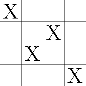
An example of a 4-by-4 Latin square sample.
This method can be extremely effective, as it quickly produces an accurate prediction without needing an initial ‘guess’, only parameter bounds. It is more computationally expensive than Metropolis-Hastings for choosing points as it maps out the whole space - but this is very small compared to the time for the MD simulation. Since it is not strictly a minimizer, we intentionally explore all of the parameter space, giving us a much better idea of where the global minimum lies, at the expense of the accuracy of the minimum position. One of the benefits of using Gaussian processes is that as well as interpolating between points, the algorithm has an estimation of the uncertainty of every point in the space too. We can build intrinsic uncertainty into the MD simulated points, essentially meaning that our interpolation does not need to exactly “fit” the point. As well as this uncertainty, we have uncertainty related to how close we are to a measured point, i.e. the further we have to interpolate, the greater our uncertainty about that value.
Gaussian Process Optimisation
Gaussian Process Optimisation (GPO) combines the ‘exploration’ of the space from the Gaussian Process Regression algorithm with the ‘exploitation’ of Metropolis-Hastings.
It starts by defining a Latin hypercube in the same way as GPR, to get an initial model of the figure of merit ‘surface’ on the parameter space.
It then proceeds via an ‘ask/tell architecture’ with an acquisition function. The acquisition function is ‘asked’ to determine what the next best point to measure at is, generally to both minimize uncertainty over the entire space as well as trying to determine the exact position of the global minimum. It is then ‘told’ what the result was, updating the model of the entire figure of merit surface.
The updating of this model adds to the computational cost of figure of merit calculation; furthermore, due to the potential large jumps between the points, a reasonable amount of equlibration of the MD simulation is likely required. That said, for noisy data where the gradient is not obtainable and the cost of obtaining the data points is large, this approach is likely to be the most efficient possible. This link to the relevant scikit docs page has more information (and some nice graphs!) on this method.