Argon A-to-Z
This tutorial aims to take the user from no familiarity with MDMC to enough competence that they can create a simple simulation and run a refinement, by walking through a simulation and refinement for the liquid argon data from van Well et al. (1985). For more details on specific parts of this, please see the how-to guides!
If you’d like to learn more about a specific object, use the Python help() command - for example help(Atom) provides information on the MDMC Atom.
We first import all of the objects we require, and set some environmental variables.
[1]:
import os
from MDMC.control import Control
from MDMC.MD import Atom, Dispersion, LennardJones, Simulation, Universe

# This setting tells MDMC how many simultaneous processes on your computer it should use
# for simulation and refinement calculations.
os.environ["OMP_NUM_THREADS"] = "4"
Setting up a configuration and simulation
We now build our Universe. For this tutorial we’re creating a cube of argon-36 atoms; our side length is 23.0668Å (angstrom), and the atoms fill it with a density of 0.0176 atoms per cubic angstrom. This simulation matches the experimental data that we’d like to refine against - you will see more about this below.
Atoms are created using MDMC Atom objects, and then the universe is filled with them via the universe.fill method.
[2]:
universe = Universe(dimensions=23.0668)

Ar = Atom('Ar[36]', charge=0.)
universe.fill(Ar, num_density=0.0176)
Universe created with:
Dimensions [23.07 23.07 23.07]
Note that at this point, there are no interaction forces between the argon atoms! The simulation doesn’t know how these atoms should interact with each other. In the cell below an appropriate (for argon) force-field interaction potential is defined; we use a dispersive interaction with potential energy calculated by the Lennard-Jones potential. This interaction has two parameters, epsilon and sigma, which determine the strength of the potential energy between atoms.
[3]:
Ar_dispersion = Dispersion(universe,  # the universe our interaction applies to
                           (Ar.atom_type, Ar.atom_type),  # the types of atoms to which it applies (only one type here!)
                           cutoff=8.,  # the cutoff distance
                           function=LennardJones(epsilon=1.0243, sigma=3.36))  # the function which calculates the potential energy between two atoms
A cutoff distance, past which atoms do not interact, is chosen arbitrarily (see help(Dispersion) for more info). A rule of thumb for Lennard-Jones is to pick cutoff=2.5*sigma. The value for argon is recommended to be between 8 and 12 ang. Ideally, and for any system you want to pick at value of the cutoff which is small while not compromising accuracy. For this system,
picking a value between 8 and 12 ang is found to give near identical results to the experimental data.
Next (and before starting the refinement), we set up the Simulation, which contains:
the
Universethat the simulation is based on;the MD engine used to run the simulations;
the time-step in femtoseconds between each simulation frame;
the temperature of the Universe (used to calculate atom velocity);
the trajectory step, which is how many time steps should occur for each ‘step’ of the refinement.
[4]:
# MD Engine setup
simulation = Simulation(universe,
                        engine="lammps",
                        time_step=10.18893,
                        temperature=120.,
                        traj_step=15)
LAMMPS (2 Aug 2023 - Update 4)
  using 4 OpenMP thread(s) per MPI task
LAMMPS output is captured by PyLammps wrapper
LAMMPS (2 Aug 2023 - Update 4)
  using 4 OpenMP thread(s) per MPI task
LAMMPS output is captured by PyLammps wrapper
Total wall time: 0:00:00
using multi-threaded neighbor list subroutines
Simulation created with lammps engine and settings:
temperature: 120.0 K
We then minimize and equilibrate the simulation; minimising the simulation avoids it getting ‘stuck’ in local minima, and equilibration runs the simulation until it reaches a state with a physically feasible temperature/energy distribution. This ensures our simulation isn’t affected by the initial arrangement of the atoms.
[5]:
# Energy Minimization and equilibration
simulation.minimize(n_steps=50)
simulation.run(n_steps=10000, equilibration=True)
Refining our data
Our simulation is now fully set up. Now we need some data to which we fit our simulation; here we use an experimental dynamic structure factor \(S(Q, \omega)\) for liquid argon. We call these dynamical properties an ‘observable’.
[6]:
# exp_datasets is a list of dictionaries with one dictionary per experimental
# dataset
# Dataset from: van Well et al. (1985). Physical Review A, 31(5), 3391-3414
# resolution is None as the original author already accounted for instrument resolution
exp_datasets = [{'file_name':'data/Well_s_q_omega_Ar_data.xml',
                 'type':'SQw',
                 'reader':'xml_SQw',
                 'weight':1.,
                 'auto_scale':True,
                 'resolution':800}]
We then need to create our parameters to fit against. In this case, we take all the universe parameters (which here are just the sigma and epsilon values that the Lennard-Jones potential depends on). Note that above when we set our initial LennardJones function in the Dispersion object, the epsilon and sigma were our “initial guesses” that the refinement will start from.
We also set constraints for our fitting parameters; we bound our sigma values to be between 2.8 and 3.8, and our epsilon to be between 0.6 and 1.4.
[7]:
fit_parameters = universe.parameters
fit_parameters['sigma'].constraints = [2.7,3.8]
fit_parameters['epsilon'].constraints = [0.5, 1.5]
Now we create our Control object. This object oversees the refinement; it brings the simulation, dataset, and the fitting parameters together, and then does the following:
Run the simulation with the current parameters.
Calculate the simulated observable from the simulation trajectory.
Compare it to the experimental observable.
Use a minimizer (optimisation process) to refine the parameters, bringing them closer to the experimental observable.
Repeat with new parameters.
The minimizer we’re using in this tutorial is CMA-ES (Covariance Matrix Adaptation Evolution Strategy)
[8]:
control = Control(simulation=simulation,
                  exp_datasets=exp_datasets,
                  fit_parameters=fit_parameters,
                  minimizer_type="CMAES",
                  reset_config=True,
                  MD_steps=4000,
                  equilibration_steps=4000,
                  data_printer='ipython',
                  file_dump_frequency="best",
                  file_dump_extent="both",
                  file_dump_loc=".",
                  file_dump_timestamped=False,
                  file_dump_prefix="mdmc_argon",
                  )
WARNING:root:`h5md_creator_name` not set, defaulting to: root
WARNING:root:`h5md_creator_email` not set, defaulting to: root@unknown
ERROR:MDMC.readers.observables.xml_SQw:
 We have set the error bar to infinity for any zero error values, this allows                 us to calculate chi-squared but effectively ignores these points, this may not                 be what you want to do, consider using a FoM which doesn't need errors i f                this is an issue

WARNING:root: The given traj_step and time_step values were not compatibile with the dataset specified.
The values (whilst prioritising time_step) have been changed to traj_step: 15, and time_step: 10.188949.
Context: for this dataset, traj_step multiplied by time_step must be ~= 152.834237 (6 d.p).

WARNING:py.warnings:/usr/local/lib/python3.12/site-packages/MDMC/resolution/resolution_factory.py:115: SyntaxWarning: Assuming energy resolution is Gaussian. To change this, input energy resolution as {'function': 'value'}, where 'function' is your desired resolution approximation function.
  warnings.warn("Assuming energy resolution is Gaussian. To change this,"
(3_w,6)-aCMA-ES (mu_w=2.0,w_1=63%) in dimension 2 (seed=776455, Mon Mar 16 13:06:46 2026)
Control created with:
- Attributes                              -
  Minimizer                           CMAES
  FoM type               ChiSquaredExpError
  Number of observables                   1
  Number of parameters                    2
Now that the dataset has been specified, and used to configure various processes and parameters, the system can be equilibrated.
[9]:
# Energy Minimization and equilibration
control.minimize(n_steps=50)
control.equilibrate(n_steps=10000)
INFO:MDMC.MD.engine_facades.lammps_engine:<class 'MDMC.MD.engine_facades.lammps_engine.LAMMPSEngine'> minimize: {n_steps: 50, minimize_every: 10, etol: 0.0001, ftol: 0.0, maxiter: 10000, maxeval: 10000}
INFO:MDMC.MD.engine_facades.lammps_engine:<class 'MDMC.MD.engine_facades.lammps_engine.LAMMPSEngine'> save_config: {n_atoms: 216}. Config saved.
INFO:MDMC.MD.engine_facades.lammps_engine:<class 'MDMC.MD.engine_facades.lammps_engine.LAMMPSEngine'> save_config: {n_atoms: 216}. Config saved.
INFO:MDMC.MD.engine_facades.lammps_engine:<class 'MDMC.MD.engine_facades.lammps_engine.LAMMPSEngine'> save_config: {n_atoms: 216}. Config saved.
INFO:MDMC.MD.engine_facades.lammps_engine:<class 'MDMC.MD.engine_facades.lammps_engine.LAMMPSEngine'> save_config: {n_atoms: 216}. Config saved.
INFO:MDMC.MD.engine_facades.lammps_engine:<class 'MDMC.MD.engine_facades.lammps_engine.LAMMPSEngine'> save_config: {n_atoms: 216}. Config saved.
INFO:MDMC.MD.engine_facades.lammps_engine:<class 'MDMC.MD.engine_facades.lammps_engine.LAMMPSEngine'> save_config: {n_atoms: 216}. Config saved.
INFO:MDMC.MD.engine_facades.lammps_engine:<class 'MDMC.MD.engine_facades.lammps_engine.LAMMPSEngine'> run: {n_steps: 10000, equilibration: True}
The number of MD_steps specified must be large enough to allow for statistically reasonable calculation of all observables. This depends the type of the dataset provided and the value of the traj_step (specified when creating the Simulation). If a value for MD_steps is not provided, then the minimum number needed will be used automatically.
Additionally, some observables will have an upper limit on the number of MD_steps that can be used in calculating their dependent variable(s). In these cases, the number of MD_steps is rounded down to a multiple of this upper limit so that we only run steps that will be useful. For example, if we use 1000 MD_steps in calculation, but a value of 2500 is provided, then we will run 2000 steps and use this to calculate the variable twice, without wasting time performing an additional 500
steps.
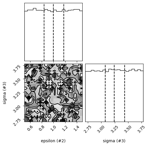
Finally, start the refinement! n_steps has been set to 25 just so you can see what a refinement looks like; it will take many more steps to fully refine a dataset. Bump it up to a higher number when you’re ready. Results can also be plotted via the control.plot_results method.
[10]:
control.refine(n_steps=25)
control.plot_results()
| FoM | CMA iteration | epsilon (#2) | sigma (#3) | |
|---|---|---|---|---|
| Step | ||||
| 0 | 3834.155100 | 1 | 1.024300 | 3.360000 |
| 1 | 3834.137662 | 1 | 1.266705 | 3.063910 |
| 2 | 3834.148672 | 1 | 1.160564 | 3.235177 |
| 3 | 3834.199753 | 1 | 0.575877 | 3.763802 |
| 4 | 3834.146209 | 1 | 0.764802 | 3.308202 |
| 5 | 3834.153174 | 1 | 1.147685 | 3.280140 |
| 6 | 3834.154144 | 1 | 1.043062 | 3.060464 |
| 7 | 3834.151844 | 2 | 0.928963 | 3.173403 |
| 8 | 3834.158371 | 2 | 1.151182 | 2.998762 |
| 9 | 3834.147126 | 2 | 1.080094 | 2.901669 |
| 10 | 3834.164155 | 2 | 1.307825 | 3.202083 |
| 11 | 3834.131081 | 2 | 1.012055 | 2.940218 |
| 12 | 3834.166865 | 2 | 1.354451 | 3.116590 |
| 13 | 3834.168184 | 3 | 1.456778 | 3.383487 |
| 14 | 3834.153490 | 3 | 0.719551 | 2.779752 |
| 15 | 3834.151736 | 3 | 1.407089 | 2.927019 |
| 16 | 3834.128015 | 3 | 0.927969 | 2.795619 |
| 17 | 3834.143115 | 3 | 0.765537 | 3.236772 |
| 18 | 3834.160023 | 3 | 0.955088 | 2.701189 |
| 19 | 3834.169934 | 4 | 0.873608 | 2.851727 |
| 20 | 3834.200968 | 4 | 1.152036 | 2.700916 |
| 21 | 3834.152984 | 4 | 0.828896 | 3.402100 |
| 22 | 3834.155170 | 4 | 0.931130 | 3.034397 |
| 23 | 3834.142580 | 4 | 0.765724 | 3.022838 |
| 24 | 3834.158134 | 4 | 0.910825 | 3.030467 |
| 25 | 3834.142941 | 5 | 1.066318 | 2.970447 |
INFO:MDMC.MD.engine_facades.lammps_engine:<class 'MDMC.MD.engine_facades.lammps_engine.LAMMPSEngine'> run: {n_steps: 3990, equilibration: False}
INFO:MDMC.MD.engine_facades.lammps_engine:<class 'MDMC.MD.engine_facades.lammps_engine.LAMMPSEngine'> save_config: {n_atoms: 216}. Config saved.
INFO:MDMC.MD.engine_facades.lammps_engine:<class 'MDMC.MD.engine_facades.lammps_engine.LAMMPSEngine'> run: {n_steps: 4000, equilibration: True}
INFO:MDMC.MD.engine_facades.lammps_engine:<class 'MDMC.MD.engine_facades.lammps_engine.LAMMPSEngine'> run: {n_steps: 3990, equilibration: False}
INFO:MDMC.MD.engine_facades.lammps_engine:<class 'MDMC.MD.engine_facades.lammps_engine.LAMMPSEngine'> save_config: {n_atoms: 216}. Config saved.
WARNING:py.warnings:/usr/local/lib/python3.12/site-packages/MDMC/refinement/minimizers/CMAES.py:202: FutureWarning: Series.__getitem__ treating keys as positions is deprecated. In a future version, integer keys will always be treated as labels (consistent with DataFrame behavior). To access a value by position, use `ser.iloc[pos]`
  last_FoM_value = last_param_row[0]

WARNING:py.warnings:/usr/local/lib/python3.12/site-packages/MDMC/control/control.py:612: UserWarning: verbose steps for process "Refinement" is set incorrectly: it is equal to 104, but the process took 129 steps.
  verbose_manager.finish("Refinement")
The refinement has not converged.

Last accepted point is:
(1.0663179280940729, 2.9704469029113767) with a minimum
FoM of 3834.142941019008.

Best point measured was:
(0.9279685845027189, 2.7956193948905) for a minimum FoM of
3834.1280147184775.


Automatic Scale Factors
data/Well_s_q_omega_Ar_data.xml  2.073609e+17
Parameter means = [2.99975266 1.01771741 3.23197607], Parameter errors = [1.15656271 0.25381442 0.30720407]
[10]: